CLHE's Triumph in Multimodal Bundle Construction Experimentation

Table of Links

Abstract & Introduction

Methodology

Experiments

Related Work

Conclusion and Future Work, Acknowledgment and References

3 EXPERIMENTS

We evaluate our proposed methods on two application domains of product bundling, i.e., fashion outfit and music playlist. We are particularly interested in answering the research questions as follow:

• RQ1: Does the proposed CLHE method beat the leading methods?

• RQ2: Are the key modules, i.e., hierarchical transformer and contrastive learning, effective?

• RQ3: How does out method work in countering the problems of cold-start items, modality missing, noise and sparsity of partial bundle? How the detailed configurations affect its performance and how about the computation complexity?

3.1 Experimental Settings

There are various application scenarios that are suitable for product bundling, such as e-commerce, travel package, meal, etc., each of which has one or multiple public datasets. However, only datasets that include all the multimodal item features, user feedback data, and bundle data can be used to evaluate our method. Therefore, we choose two representative domains, i.e., fashion outfit and music playlist. We use the POG [11] for fashion outfit. For the music playlist, we use the Spotify [7] dataset for the bundle-item affiliations, and we acquire the user feedback data from the Last.fm dataset [2]. Since the average bundle size is quite small in POG (it makes sense for fashion outfit), we re-sample a second version POG_dense which has denser user feedback connections for each item. In contrast, the average bundle size in Spotify dataset is large, thus we sample a sparser version Spotify_sparse, which has smaller average bundle size. To be noted, we keep the integrity of all the bundles in all the versions, which means we do not corrupt any bundles during the sampling. For each dataset, we randomly split all the bundles into training/validation/testing set with the ratio of 8:1:1. The statistics of the datasets are shown in Table 1. We use the popular ranking protocols of Recall@K and NDCG@K as the evaluation metric, where K=20.

3.1.1 Compared Methods. Due to the new formulation of our work, there are no previous works that have exactly same setting with ours. Therefore, we pick several leading methods and adapt them to our settings. For fair comparison, all the baseline methods use all the three types of extracted features that are same with our method. In addition, they all use the same negative log-likelihood loss function.

• MultiDAE [51] is an auto-encoder model which uses an average pooling to aggregate the items’ representations to get the bundle representation.

• MultiVAE [31] is an variational auto-encoder model which employ the variational inference on top of the MultiDAE method.

• Bi-LSTM [21] treats each bundle as a sequence and uses bidirectional LSTM to learn the bundle representation. • Hypergraph [54] formulates each bundle a hyper-graph and devises a GCN model to learn the bundle representation.

• Transformer [3, 46] tailors a transformer to capture the item interactions and generate the bundle representation.

• TransformerCL is the version that we add bundle-level contrastive loss to the above Transformer model.

3.2 Overall Performance Comparison (RQ1)

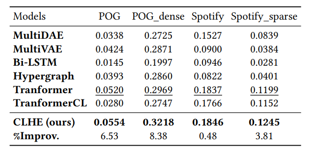
Table 2 shows the overall performance comparison between our model CLHE and the baseline methods. We have the following observations. First, our method beats all the baselines on all the datasets, demonstrating the competitive performance of our model. Second, over the baselines, Transformer and TransformerCL achieve the best performance, showing that the self-attention mechanism and contrastive learning can well preserve the correlations among items within the bundle, thus yielding good bundle representations. Third, comparing the results between different versions of dataset, we find that: 1) the performance on POG_dense is much larger than that on POG due to denser user-item interactions, demonstrating that user feedback information is quite helpful to the performance; 2) the performance of Spotify_sparse is relatively smaller than that on Spotify since the sparser bundle-item affiliation data, justifying our hypothesis that large-scale and high-quality bundle dataset is vital to bundle construction. Finally, we have an interesting observation that the performance improvements on the four datasets is negatively correlated with "#Avr.B/I", as shown in Table 1, in another word, in scenarios that items are included in fewer bundles (i.e., the dataset include more sparse items), our method performs even better. This phenomenon further justifies the advantage of our method in countering the issue of sparse items.

3.3 Ablation Study of Key Modules (RQ2)

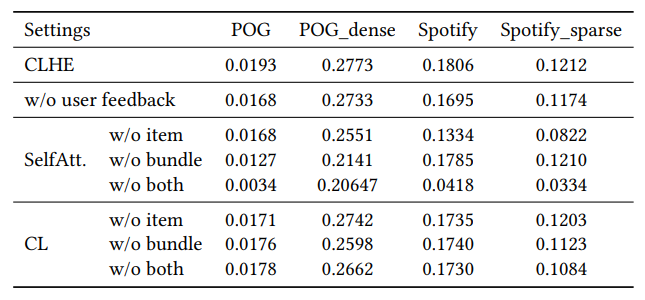
To further evaluate the effectiveness of the key modules of our model, we conduct a list of ablation studies and the results are shown in Table 3. First and foremost, we aim to justify the effectiveness of the user feedback features. Thereby, we remove the user feedback features from our model (i.e., remove p𝑖 from f𝑖 ) and build an ablated version of model, i.e., w/o user feedback. According to the result in Table 3, after removing user feedback features, the performance reduces clearly, verifying that user feedback feature is significant for bundle construction. Second, we would like to evaluate whether each component of the hierarchical encoder is useful. We progressively remove the two self-attention modules from our model and replace them with an vanilla average pooling, thus yielding three ablated models, i.e., w/o item, w/o bundle, and w/o both. The results in Table 3 show that the removal of either selfattention modules causes performance drop. These results further verify the efficacy of our self-attention-based hierarchical encoder framework. Third, to justify the contribution of contrastive learning, we progressively remove the two levels of contrastive loss, thus generating three ablations, i.e., w/o item, w/o bundle, and w/o both. Table 3 depicts the results, which demonstrate the both contrastive losses are helpful, especially on the sparser version of datasets.

3.4 Model Study (RQ3)

To explicate more details and various properties of our method, we further conduct a list of model studies.

3.4.1 Cold-start Items. One of the main challenges for bundle construction is cold-start items that have never been included in previous bundles. It is difficult to directly evaluate the methods solely based on cold-start items since there are few testing bundles where both the input and result partial bundles purely consist of coldstart items. Nevertheless, we come up with an alternative way to indirectly test how these methods perform against cold-start items. Specifically, we remove all the cold-start items and just keep the warm items in the testing set, i.e., the warm setting. We test our method and all the baseline models on this warm setting. The results shown in Table 4 illustrate that: 1) the performance of all the models on the warm setting are much better than that of the warm-cold hybrid setting (the normal setting as shown in Table 2), exhibiting that the existence of cold-start items significantly deteriorate the performance; and 2) the performance gap between CLHE and the strongest baseline in the hybrid setting is obviously much larger than that on the warm setting, implying that our method’s strength in dealing with cold-start items.

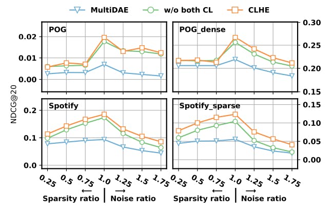
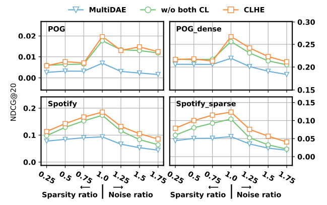
3.4.2 Sparsity and Noise in Bundle. Another merit of our approach is that the contrastive learning is able to counter the sparsity and noise issue when the input partial bundle is incomplete. To elicit this property, we corrupt the testing dataset to make the input partial bundle sparse and noisy. Specifically, we randomly remove certain portion of items from the input partial bundle to make them sparser. To make the partial bundle more noisy, we randomly sample some items from the whole item set and add them to the bundle. Then we test our model and the model without both levels of contrastive loss, and the performance curves are shown in Figure 3, where the x-axis is the ratio of bundle size after corruption compared with the original bundle, and the ratio=1 corresponds to the original clean data. From this figure, we can derive the conclusion that: 1) with the sparsity and noise degree increasing, both our method and baselines’ performance drops; 2) our method still outperforms baselines even under quite significant sparsity or noise rate, such as removing 50% seed items or adding 50% more noisy items; and 3) the contrastive loss in our model is able to combat the parse and noise bundle issue to some extent.

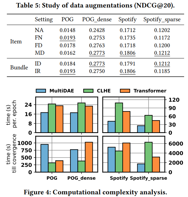
3.4.3 Data Augmentations. Data augmentation is the crux to contrastive learning. We search over multiple different data augmentation strategies at both item- and bundle-level contrastive learning, in order to find the best-performing setting. In Table 5, we present the performance of CLHE under various data augmentations at both item- or bundle-level. Overall speaking, data augmentation methods may affect the performance and proper selection is important for good results.

3.4.4 Computational Complexity. Self-attention calculates every pair of instances in a set, i.e., features of an item or items of a bundle, thus it usually suffers from high computational complexity. We record the time used for every training epoch and the time used from the beginning of training till convergence, and the records of our method and two baselines, i.e., MultiDAE and Transformer, are illustrated in Figure 4. The bar chart reveals that on the one hand, our method is computationally heavy since it takes the longest time for each training epoch; on the other hand, our method takes the least training time to reach convergence on three datasets. In conclusion, our method is effective and efficient during training, while the inherent complexity induced by hierarchical self-attention may impose the inference slower. We argue that various self-attention acceleration approaches could be considered in practice, which is out of the scope of this work.

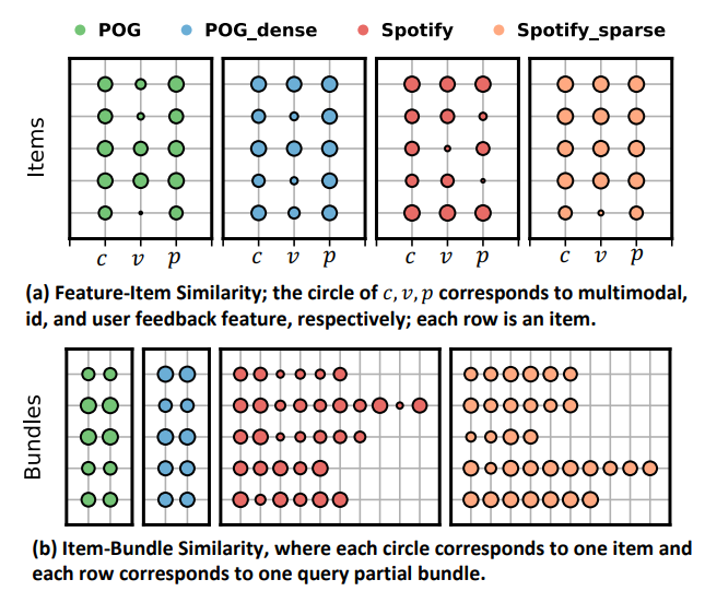
3.4.5 Case Study. We would like to further illustrate some cases to portrait how the hierarchical encoder learn the association of multimodal features and the multiple items’ representations. Specifically, for both item- and bundle-level self-attention modules, we take the last layer’s output representation as each feature’s (item’s) representation, and calculate the cosine similarity score with the whole item (bundle). We cherry pick some example items and bundles, as shown in Figure 5. The results of feature-item similarity exhibit that the three type of features could play distinctive roles in different items, showing the importance of all the three types of features. For the item-bundle similarity results, we can find that items do not equally contribute to their affiliated bundles, thus it is crucial to model the bundle composition patterns. Here we just intuitively illustrate some hints about the bundle representation learning, more sophisticate analysis, such as feature pair or item pair co-effects, is left for future work.

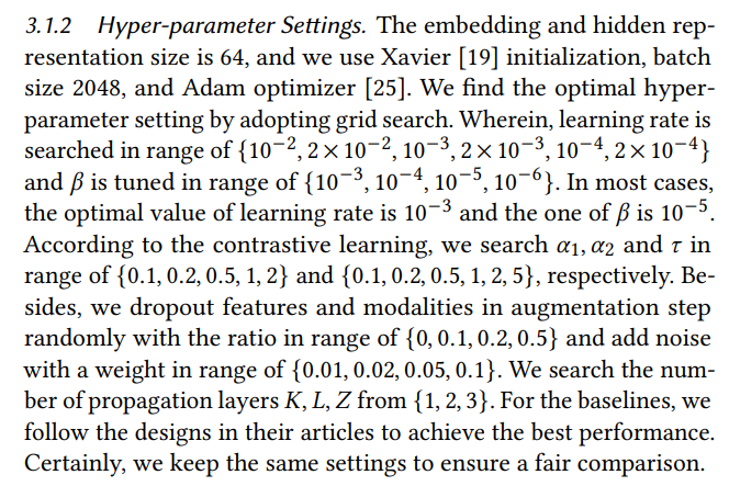
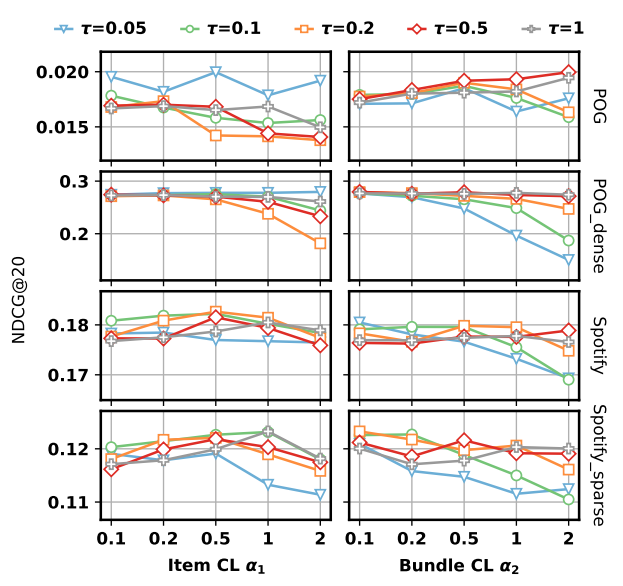
3.4.6 Hyper-parameter Analysis. We also present the model’s performance change w.r.t. the key hyper-parameters, i.e., the temperature 𝜏 in contrastive loss and the weights 𝛼1, 𝛼2 for the two contrastive losses. The curves in Figure 6 reveal that the model is still sensitive to these hyper-parameters, and proper tuning is required to achieve optimal performance.